Transactional Storage

In this blog we are going to talk about databases, as a developer we do not care about the internal of database, but we do care about choosing a suitable database for your workload and finetuning it for performance, to do that we need to have a rough idea of how databases work under the hood.

Simple Database

First, let's build the world's simplest database to store key-value data with just two operations:

• Store a key-value pair by appending to the end of a file.

• Get the value given the key from database by searching matching line, extract the value of the matching keys, and return the latest.

This simple setup is surprising efficient for small scale data, because appending to a file is generally a fast operation. However, it is also obvious that this database does not perform well when the amount of data grows very large. The following table shows some statistics of this simple database with a naive implementation on my machine [ref].

Operation	Speed
write 10,000 records	0.0042s
write 100,000 records	0.0433s
write 1,000,000 records	0.5262s
read 1,000 random records from 10,000 records	0.0890s
read 1,000 random records from 100,000 records	0.9261s
read 1,000 random records from 1,000,000 records	10.0677s

Index

As we saw, our write queries are pretty efficient, but our read queries slow down drastically as our database grows. In order to efficiently find value of a given key, we can use an index. An index is a data structure derived from the primary data, storing additional metadata that speed up read queries, avoid the need of scanning the full database.

HashMap

A index can be just a simple hash map mapping key to byte offset of the value in the database. With this simple setup, we can achieve 10-100x faster reads, trading with ~2x slower writes. This is an important trade-off --- while an well-chosen index speeds up reads, it always slows down writes, because we have an additional data structure to update every time we do a write.

Operation (hash map index)	Speed
write 10,000 records	0.0084s
write 100,000 records	0.0897s
write 1,000,000 records	1.1117s
read 1,000 random records from 10,000 records	0.0023s
read 1,000 random records from 100,000 records	0.0134s
read 1,000 random records from 1,000,000 records	0.1794s

This simple setup [ref] is essentially what Bitcask does --- the default storage engine of Riak [ref]. It offers high performance reads and writes, given the index must fit in available RAM, because the index must be loaded into memory. If the data is already present in the file system cache, it does not even require a disk access on read. In the case where your index can't be loaded into memory, you can use alternative like Berkeley DB which designed to operate directly on disk. If you are thinking about on disk hash map, that is too expensive, we cannot easily expand by rehashing or resolve hash conflicts.

LSM-Tree

We have just made a high performance database, but we also need to store as many data as possible. An obvious issue with our simple database setup is our append-only data file (a.k.a. log) just grows indefinitely, we are appending an additional value for every new write, leaving the stale data on disk, this will eventually consumes all available memory. One solution would be during write, find and replace old value, leaving no duplicate in the log. This option is viable but in this section, we are going to focus on another way of solving this problem: removing stale data occasionally in the background. This leads us to a family of databases based on the Log-Structured Merge-Tree (LSM-Tree).

Compaction

The process of removing stale data is called compaction. Stale data are outdated duplicated keys exists in the log. One simple way to remove these keys would be go through all entries from latest to oldest, adding keys to a hash set and remove entries with keys already exists. This works only if all keys fits into memory as this uses O(n) space.

Let's do better by making one change to our log: make it sorted. Sorted data groups duplicates by key naturally and we can go through the entries once and remove duplicates without using additional space, resulting in a O(1) space algorithm. We will also split the log into multiple smaller data files (a.k.a segments), and run compaction on subset of the segments to avoid scanning through too many data at once.

You may have notice maintaining a sorted data structure would means our write becomes O(logn). This is true but it is faster than you might think. In practice, a write usually consists of insert data into an in-memory data structure called memtable, typically implemented with b-tree or skip list, providing fast write. This memtable will be flushed to disk as an immutable data file after reaching certain size, and this immutable on disk memtable is called Sorted String Table (SSTable). Since our memtable can only grow to a pre-determined size in the memory (let say 4mb), the n in our log(n) complexity is fairly small, and it is very efficient.

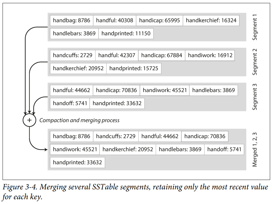
Merge

We just came up with an efficient way to clean up duplicates in the database by splitting and merging our log file. But we introduced another problem at the same time: as more and more SSTables will be created, our reads will get slower too! This is because during a read operation, if data is not present in the memtable, we will need to utilize SSTables on disk. While we can make use of bloom filter to reduce the number of SSTables to check, we generally needs to scan the SSTables linearly, this hurts performance over time as we have more SSTables. Therefore after compacting multiple segments, we should merge them to prevent over-fragmentation.

This merge process is pretty straight-forward, since each of our segments are sorted, this becomes a merge-k-sort-array leetcode problem. The nice thing about this process is, if you think about it a little bit, it can be done together with compaction in one step in the background because SSTables are immutable, this means we can still serve read requests while merging the segments in the background.

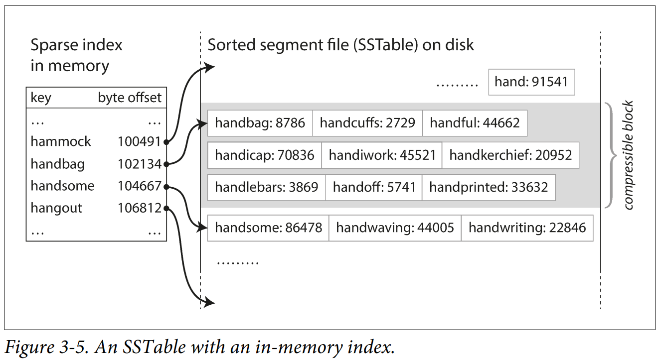
When searching within each SSTable you still need to have an index in memory to allow you to quickly locate the entry you are looking for, but it can be sparse because data is sorted and scanning through a few kilobytes can be done a short time. You might ask since the data is sorted why not binary search? This is because as a key-value store, values often comes in variable length, it is difficult to tell where a entry starts and ends without an index, we also want to reduce the amount of disk access as much as possible.

LSM

The procedure we just describe is essential how LevelDB [ref] and RocksDB [ref] works under the hood for reads and writes. Lucene, a full-text search engine used by Elastic Search uses a similar method for storing its term dictionary where it maps a term to all document ids where this term appeared in a key-value store.

There are a great amount of details we did not cover in this section, let's have a brief overview on other important bits.

• Deletion A special entry (sometimes called tomestone) is written as an indicator to invalidate all previous entries of that key.
• Crash Recovery So we have transformed our initial log into memtables and SSTables, but we still need to append data to a special log before inserting into memtable, called Write-Ahead Log (WAL). This log allow database to replay data lost in memory during crash recovery. In case of partially written entry in WAL, data validation like checksums is used to ensure only fully written entries are replayed.
• Concurrency Control Since writes are appended to WAL in strictly sequential order, a common implementation is to have only one writer thread, but since disk write is sequential, it is enough to provide remarkably high throughput. Read can be concurrent because SSTables are immutable.

You might say this whole idea based on append-only log is too wasteful, actually, it is. We need to do additional work to compaction and merge the database. However, people have not come up with a perfect structure that solves all the problems, again this is a trade-off we have to make. In practice, the LSM structure is simple and effective. When compared to hash index, it brings several benefits:

• Memory LSM-tree does not requires all keys to be fitted into memory.
• Disaster Recovery Disaster recovery becomes simple as you do not need to worry about partially written SSTables due to its immutability. Note we need to rebuild all the sparse indices for SSTables in memory if we want to restart the database, which can be time-consuming.
• Cost Compaction and merge simply go through data sequentially, can be done efficiently.
• Ranged Queries You can easily scan related keys for example from Kitty000 to Kitty999 efficiently since keys are sorted.

LSM-tree databases are not perfect, you might have already recognize a problem with LSM-tree setup --- looking for a missing key can be inefficient because you need to look at the memtables, then all the SSTables filtered by bloom filters. Compaction can also interfere performance of ongoing writes, although database tries to do so without affecting cocurrent access, some strategies for determining the order and timing of how SSTables are compacted and merged includes level-tier, used in LevelDB and RocksDB, and size-tier, used in HBase, Cassandra supports both.

B-Tree

The log-structured index is gaining popularity in recent years, but the most widely used index is quite different --- B-tree. Similar to LSM-tree, B-tree arrange written data in sorted order, but apart from this, there is rarely any similarity, it has a different design philosophy.

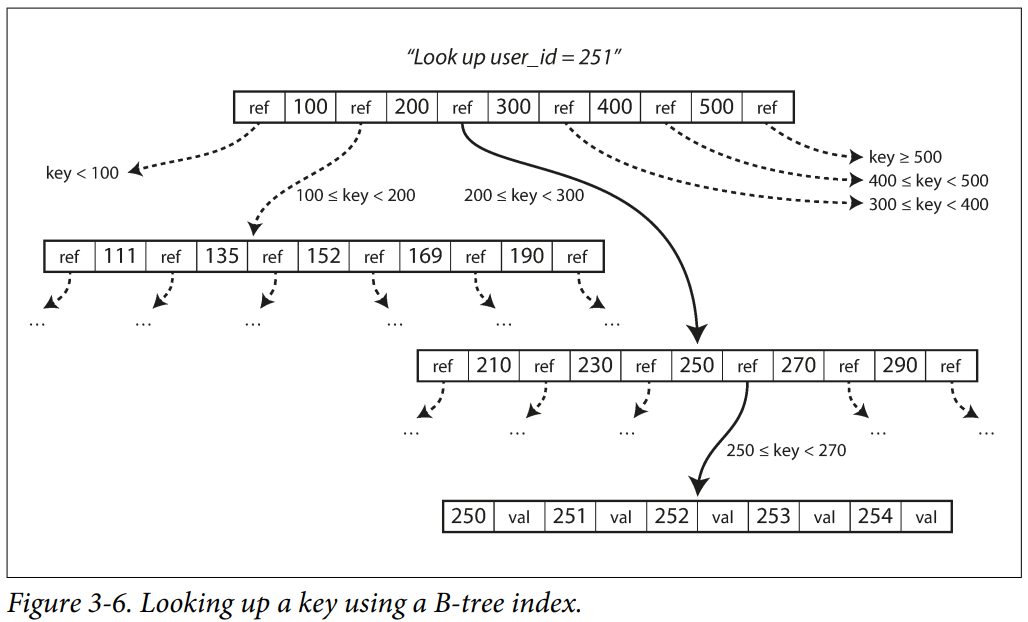
In a key-value store, B-tree breaks down its value into fixed size blocks (or pages). This align more closely with underlying hardware, as disks are also arranged in fixed size blocks. These pages are identified with an unique address, and a page may not only contain data, it can also contain a range of addresses, allowing it to reference to other pages.

When given a key to read, we starts from a designated root page, find the reference of the range of keys which the given key falls into, then navigate to that page, we do this recursively until we reached a leaf page, which contains the data in-place (if it is small enough, a.k.a. clustered index) or a reference to the address of the block of data.

Write is also navigate down the tree in similar fashion, except that we either to insert or update the value. When a page get large enough, an insertion could trigger a page split, to do this we need to split a full-page into two half-full pages and update their parent reference. This is a dangerous operation, because it is a two step process. We could ended up with partially written pages in the case of sudden failure.

Reliable Reads and Writes

We can again use a write-ahead-log (WAL) to keep track of every b-tree modification before it is applied to the tree itself, we can use this log to bring b-tree back to a consistent state. Instead of using WAL, some databases also use a copy-on-write scheme, every time a write is needed, it create a new version of the parent page, containing new references to new data. As we will see in later blog, it is useful for concurrency control.

Apart from write itself, a two step process can also result in us reading the b-tree in an inconsistent state if we have concurrent read and write. This is typically resolved using latches, a light-weight lock apply to part of the tree.

Comparison

LSM-tree typically can sustain higher throughput compared to b-tree, this is because it is less vulnerable to write amplification. Write amplification refers to a scenario which one write operation often leads to multiple writes to the disk. This can happen due to internal operations of the database, such as existence of WAL, compaction, indexing and copy-on-write scheme. For write intensive application, increased disk write consumes more I/O bandwidth, leading to slower write performance. For SSDs it is more concerning because it can only sustain a limited amount of writes before tearing out. This is particular a problem for b-tree because it updates value in-place rather than writing sequentially to new address like LSM-tree.

On the other hand, since index can exists in one place, which makes b-tree appealing to databases that offer strong transactional semantics, where locks can be applied directly on the tree to a ranged of keys. A tree structure also allow it to offer faster and more consistent read, while a read in LSM-tree is required to look into multiple places such as memtables and SSTables.

Other Indices

Multi-column Indexes

So far we have only discussed key-value index, which maps a single key to value. However, it is quite common we want to query across multiple columns. For example, a restaurants search website may needs to find all restaurant within a certain latitude and longitude. A standard b-tree or LSM-tree is not able to answer this type of question. One option is to translate a two-dimensional value into one-dimensional using a space-filling curve, then use a regular b-tree index, or more commonly, specialized index such as R-tree is used [ref].

Full-text Search and Fuzzy Index

Sometimes we might want our database to support searching for documents containing a certain word. This translate to a range of indices with similar keys, or even 1 edit distance away, regardless of grammatical variation of the word. As we saw in previous section, Lucene is one example of such full-text search engine. In Lucene, index is a finite state machine over characters in the keys, it can be transformed into Levenshtein automation, which allow efficient searching for words within a given edit distance away.

In-memory Only

The data structures we discussed so far are answers to limitation of disk. Disks are awkward to deal with, it needs to be lay out carefully for efficient reads and writes. However, we tolerate them because disks are durable and cheaper than RAM. But over the years RAM has become cheaper and some datasets are not that big, making them quite feasible to store entirely in memory.

There are already well-known in-memory caches out there, like Redis [ref] and Memcache [ref]. The main difference between in-memory cache and in-memory database is really just a matter of persisting on disk as backup and reloading into memory on start-up.

Counterintuitively, in-memory databases are faster not because they do not need to write or read from disk, even a disk-based database might not frequently access disk either because the dataset is small enough, or it is cached by the OS. The performance advantage comes from not needing to translate its in-memory data structure into a representation suitable to be written to disk.